Ray casting or ray tracing dates back to the '90s computer games as a technique of producing realistic 3D environments, although, according to Wikipedia, it was invented by Albrect Dürer already in the 16th century. No computers back then, though. While the two terms are, at times, used interchangeably, ray casting has also been described as a predecessor to recursive ray tracing.
With the limited computing power available, the first ray casting games (remember Wolfenstein 3D or Doom?) generally "cast rays" only on a horizontal level. The environment was thus not truly 3D, but only appeared to be, when moving on a flat surface. There are ways to emulate jumping or kneeling, or looking up or down, but they are not true 3D - which might not matter much in a heated game play.
The basic premise is simple: Say you have a display 800 pixels wide. Cast 800 rays horizontally, e.g. from left to right, and see what the rays hit first - in the simplest case, a wall. Then assume that wall goes from floor to ceiling, and draw the one vertical line (one pixel wide) of that wall. Do the same for each of the 800 rays, and you have filled the screen with a ray cast 3D space.
I got my inspiration to try this from raytomely's ray casting routine where he kindly also points to a step-by-step guide by F. Permadi, written already in 1996. This v0.5 is only a half-product - it does cast the rays and illustrates the technique by drawing a map with the rays, but it does not (yet) do the actual drawing of the 3D space. That will follow in a later version and post.
As usual, the Python code relies on PyGame and NumPy and can be found in my GitHub repository.
Looping the loop
Computers are fast, but if you need to do almost the same thing many, many times (like calculating the 800 rays 60 times a second), the processing costs start to add up. The basic approach is to write a loop, with changing parameters (like the number of the ray going from 1 to 800 ), to process each case in its turn. In the 1990's, this was about as much you could do about it - although people (like myself) spent days optimizing those costly loops in
Assembly language. These days, Assembly is rarely used, but the hardware helps you with all kinds of neat stuff like multiple cores, real parallel processing, and caches, not to mention graphics cards. But - if you want fast code, Python is really not your best choice. The processing cost (overhead) of running a Python loop is enormous. Really. The best solution would be to use another language, at least for the loop. Another, and much more efficient when it comes to
your time i.e. the time it takes to develop the code, is to use a Python module which can run those loops for you in a more efficient way. I have been using
NumPy and, as it's easier to stick with something you know at least something about, am using it here as well. The principal idea is not to run a loop in Python but to ask for as much calculations and data as possible from NumPy in one go; for example, instead of running a loop 800 times and calculating a sine for an angle etc. every time, asking NumPy to return an array of sines for all 800 angles in one instruction.
To help and limit the amount of checking when the ray hits the wall, the walls are based on a grid. In the image below you can see the grid and the wall blocks, and all the rays from the viewer (the blue ball) in yellow. It is thus sufficient to check if the ray hits a wall at only the points where it crosses the grid. In the basic algorithm (see
F. Permadi), the grid crossings are checked one by one in a loop, and if the ray does hit a wall, the loop is exited - there's no need for any further checks. To avoid the loop, I am checking all the crossings at once. In the other image with red and green circles, the circles represent the checked points (note that only ten rays instead of all 800 are shown).
 |
| Casting yellow rays from the blue dot (viewer). |
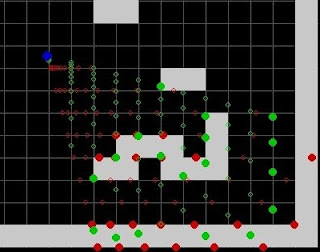 |
| Showing the horizontal (green) and vertical (red) grid crossings for selected rays. A big, filled circle means hitting a wall. |
Casting exercise
How to go about this, then? Below is the part preparing the calculations; e.g. self.width = 800, representing the number of rays, self.view_blocks = 10, giving the maximum distance in grid blocks for viewing, and self.view_width = 60, the width of the viewer's field of vision in degrees. Note all of these values are just examples and could be defined freely.
    def raycast(self, screen, block_size):

        # go through view horizontally i.e. from position and view_angle go from left view_angle_witdh / 2 to right view_angle_witdh / 2.
        # below "horizontal" and "vertical" refer to a map on the screen, not the view itself.
        # angle 0 degrees = "up", rotation clockwise

        # position rounded to grid and the decimals (ie. position within the grid it is in)
        pos = np.floor(self.position)
        pos_dec = self.position - pos

        width = self.width  # this is the number of rays cast - ideally the width of the program window in pixels, so one ray per vertical line of pixels.
        view = self.view_blocks  # nr of blocks: how far is visible (and, hence, how far must be calculated)
        rng_width = np.arange(width)
        # rng_view goes from zero to maximum view length in blocks.
        rng_view = np.arange(view + 1)  # add 1 to make sure covers the viewable distance as blocks are "rounded down"
        # calculate all angles etc. in one go - faster than looping
        # rads is an array (size: width) of all view angles in radians. Add 0.0001 to avoid exact 0/90/180/270 deg (and hence 0 sin/cos - div by zero)
        # rads are not evenly spaced, as they are on a line, not a circle radius. Their tangent is evenly spaced (when view_angle not yet applied),
        rad_tan = np.tan(self.view_width * np.pi / 360)  # rad_tan is the tangent of half the viewing angle
        rads = np.arctan((rng_width / (width - 1) - 0.5) * rad_tan * 2) + self.view_angle * np.pi / 180 + 0.0001
        sin_a = np.sin(rads)
        cos_a = np.cos(rads)
        tan_a = np.tan(rads)
        sign_x = np.sign(sin_a)   # sign_x = +1 for angles > 0 and < 180, -1 for angles > 180
        sign_y = np.sign(cos_a)   # sign_y = +1 for angles < 90 or > 270, -1 for angles > 90 and < 270

        # get the first encountered coordinates when moving to next grid along ray line
        # if sign_y is negative, ray is cast downwards and the y distance is pos_dec[1] - 1. The same for x...
        x_first = (pos_dec[1] + (sign_y - 1) / 2) * tan_a
        y_first = (pos_dec[0] - (sign_x + 1) / 2) / tan_a
Above,
rads represent all the angles (in radians) I want to cast rays to, and
sin_a,
cos_a, and
tan_a the
sine, cosine, and tangent of those angles; each is a NumPy array of 800 elements. I also need to define the sign in both x and y coordinates the ray is going to (up and left being negative, down and right positive), and the distance to the first grid crossing in both x and y.
Continuing to define the vertical crossings (red circles in the image above):
        # vertical intersections of ray and grid; y coordinate increases/decreases by one, calculate respective x coordinate
        # x_coord_y is the "grid point" (no info on which side of grid) while x_coord_y_adj is the y coordinate adjusted for viewer position relative to it (includes side).
        #   i.e. if grid point is higher than viewer (sign_y = -1), 1 is added to bring x_coord_y_adj to the bottom of that grid point.
        vert_grid_range = rng_view
        x_coord = self.position[0] + x_first[:, None] + vert_grid_range * (sign_y * tan_a)[:, None]
        x_coord_y = pos[1] - (vert_grid_range + 1) * sign_y[:, None]
        x_coord_y_adj = x_coord_y - (np.sign(x_coord_y - pos[1]) - 1) / 2
        # get the respective grid cell data from the map. Make sure not to exceed map boundaries. Pick only "view" nr of blocks; then add a "stop block" as last block
        vert_grid = np.hstack((
            self.map_array[(np.minimum(np.maximum(x_coord[:, :view], 0), self.map_size[0] - 1)).astype(np.int16),
                           (np.minimum(np.maximum(x_coord_y[:, :view], 0), self.map_size[1] - 1)).astype(np.int16)],
            np.ones((width, 1), dtype=np.int16)  # this is the farthest block and always marked as "1" to make sure argmax finds something.
            ))
        # find the first nonzero item's index for each angle. Since distance is growing with each item, this is the closest wall encountered for each ray.
        vert_grid_first = (vert_grid != 0).argmax(axis=1)
        # construct an array of grid item, side (0 = up, 1 = right, 2 = down, 3 = left) map x, map y, and distance from viewer
        vert_data = (np.vstack((
            vert_grid[rng_width, vert_grid_first],
            sign_y + 1,
            x_coord[rng_width, vert_grid_first],
            x_coord_y_adj[rng_width, vert_grid_first],
            np.abs((x_coord[rng_width, vert_grid_first] - self.position[0]) / sin_a)
            ))).transpose()
The range x_coord on the grid is, from the viewer position, the distance to the first crossing x coordinate (x_first) plus a multiple of (sign_y * tan_a), which is the difference in x coordinates when we move from one vertical grid line to the next. Note that the multiples are between 0 and 10 here, so we get 11 crossings for each ray - 800 x 11 = 8,800 x_coord in total. (Why 11 instead of 10? I have defined 10 as the maximum viewable distance, and the first grid crossing might be very close - hence 10 + 1 are needed to cover the distance of 10.)
The y coordinates (x_coord_y) of these crossings are, by definition, on the grid, but since the direction (sign_y) can be either -1 or +1, they are calculated for all 800 rays as well.
Being on the grid does not really tell us yet which side of the grid block we are seeing - it could be the "upper" side (if we are looking "down") or vice versa. x_coord_y_adj adjusts the coordinate using the direction (sign_y).
Next, I need to figure out if those vertical grid crossings are hitting walls or not. The self.map_array is a simple array of block types; so far I only have defined "0" (empty) and "1" (wall). The vert_grid is picking the block type from the self.map_array, using np.minimum and np.maximum to keep within the map at all times. In effect, in vert_grid I have 800 rows (rays) and 11 crossings for each row, and for each either 0 or 1 indicating whether there's a wall or not. Using np.hstack I add a 12th item to each ray with a 1 to make sure argmax next has a wall to find.
Now we have an array containing all rays (800 rows) and the first 11+1 vertical grid crossings. I need to find the first one which is not empty (i.e. is a wall). For that I use (vert_grid != 0).argmax(axis=1) which first converts the vert_grid to an array of True or False values (required in the future if there are more wall types), and then returns the index of the first encounter of the maximum value (always True) on each row. That's the closest wall.
Then I construct an array of the 800 rays, consisting the data I later need for drawing it: grid item (wall type), side (0 = up, 1 = right, 2 = down, 3 = left), x, y, and distance from viewer.
Next, I do the exact same thing with horizontal crossings (green circles in the image above), just switching the axes. What remains is to figure out, for each ray, whether the closest wall found was from the vertical crossings or the horizontal crossings:
        # combine data on vertical and horizontal first encountered walls
        comb_data = np.stack((vert_data, horiz_data))
        # find the closest of these two - distance being item 4
        comb_closest = np.argmin(comb_data[:, :, 4], axis=0)
        # pick these for the closest data
        self.ray_data = comb_data[comb_closest, rng_width, :]
I combine the data on vertical and horizontal first encountered walls to a new array and pick, again for each ray, the one with minimum distance to viewer, using np.argmin and the distances stored. Now self.ray_data has the same data as vert_data and horiz_data, but only the closest wall for each ray.
What remains is drawing the map and the viewer, with the area the viewer can see.
Running the code, the user can steer the viewer with the cursor keys. Use m key to switch viewing mode between the yellow area and green and red circles, as in the two images above.


this is awesome
ReplyDeletenice
ReplyDeletenais
ReplyDelete